Governing equations for the physics of the engineering problems generally consists of the differential equations. Finding an analytical solution for a differential equation can be difficult and in some cases even impossible. That’s why engineers mostly use computational methods to solve complex problems. Finite difference method is the most basic method among computational methods. In this post, I will give brief information about the finite difference method and share a finite difference code prepared with MATLAB for a 2D steady state heat conduction problem.
Let us take the 2D steady state heat conduction problem from “Fundamentals of Heat and Mass Transfer” book (Problem 4.2), which is shown in Figure 1. Since the boundaries of the plate have fixed temperature values, the first type or Dirichlet boundary conditions apply to this problem.

According to the problem, we will try to determine the temperature at the midpoint of the rectangular plate. Equation 1 is the heat equation in 2D cartesian coordinates with constant thermal conductivity.
(1) ![]()
Since this is a steady state problem, ![]() term and hence the right-hand side is equal to zero. Besides, there is no heat generation in the plate. Therefore Equation 1 simplifies to Equation 2, which is Laplace’s equation.
term and hence the right-hand side is equal to zero. Besides, there is no heat generation in the plate. Therefore Equation 1 simplifies to Equation 2, which is Laplace’s equation.
(2) ![]()
A finite difference grid for an arbitrary domain is shown in Figure 2. Laplace’s equation can be discretized with the second-order central difference scheme in accordance with Figure 2 is given in Equation 3. Please note that, if step size is selected as ![]() Equation 3 simplifies to Equation 4.
Equation 3 simplifies to Equation 4.

(3) ![]()
(4) ![]()
In order to solve the problem, the domain should be discretized with appropriate step sizes in x and y directions and Equation 3 should be written for all nodes, except the boundary nodes. Because we need to have neighbor nodes when using Equation 3 and boundary nodes have one or two absent neighbors. For example, if we would consider the node on the top left of the rectangle as ![]() , there would not be a
, there would not be a ![]() and a
and a ![]() for that node. In that way, we could not have used Equation 3 for the solution. One may solve a domain including boundary nodes with Neumann or Robin boundary conditions, but the solution with these boundary conditions requires different formulations than Equation 3.
for that node. In that way, we could not have used Equation 3 for the solution. One may solve a domain including boundary nodes with Neumann or Robin boundary conditions, but the solution with these boundary conditions requires different formulations than Equation 3.
The matrix formulation for the solution of Equation 3 is in the form of ![]() , where
, where ![]() is finite difference coefficient matrix,
is finite difference coefficient matrix, ![]() is the unknown vector, and
is the unknown vector, and ![]() is the right-hand side vector. A good practice may be writing the temperature values of the boundary nodes to the right-hand side matrix instead of finite difference coefficient matrix. In this way, the finite difference coefficient matrix will be a banded matrix with the same elements on each band. On the other hand, the right-hand side vector will consist of zero elements except for the elements that correspond to the nodes adjacent to the boundaries. Once the matrices have been constructed, the unknown vector can be calculated simply by taking inverse the finite difference matrix and multiplying it by the right-hand side vector.
is the right-hand side vector. A good practice may be writing the temperature values of the boundary nodes to the right-hand side matrix instead of finite difference coefficient matrix. In this way, the finite difference coefficient matrix will be a banded matrix with the same elements on each band. On the other hand, the right-hand side vector will consist of zero elements except for the elements that correspond to the nodes adjacent to the boundaries. Once the matrices have been constructed, the unknown vector can be calculated simply by taking inverse the finite difference matrix and multiplying it by the right-hand side vector.
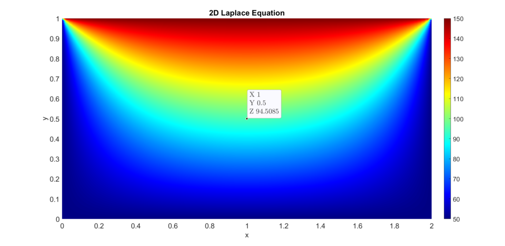
The solution of the problem is provided as ![]() in the book. The result obtained with the finite difference code is shown in Figure 3.
in the book. The result obtained with the finite difference code is shown in Figure 3.

It can be seen that the solution provided in the book and the solution obtained with the finite difference code are nearly the same. Please note that this code does not use an iterative approach. Therefore, its accuracy is dependent on step size and the order of the derivative approximation. Download link for the finite difference code is given below.
2D Laplace’s Equation FDM Solver for a Rectangular Plate
References
[1] Bergman, T. L., Incropera, F. P., DeWitt, D. P., & Lavine, A. S. (2011). Fundamentals of heat and mass transfer. John Wiley & Sons.